Part I: The Batsman's Engine

The "Good Shot" Paradox

Consider a classic scenario: Virat Kohli is facing Starc in the 18th over of a T20 chase. Starc bowls a length ball outside off. Kohli plays a lofted Cover Drive.

In traditional analytics, we look at the outcome: Did it go for 4? Did he get out? If he scored, it was a "good shot." If he got caught, it was a "bad shot."

But this binary view is flawed. As analysts, we should ask: What was the Expected Value of that decision before the ball left the bat?

Was it physically the right shot for that line and length?
Did the field placement justify the risk?
How much did the match pressure influence the execution error?

Existing metrics like Strike Rate and Average are retrospective they tell us what happened. I wanted to build something predictive. I wanted to quantify the Intent, the Physics, and the Context of every single delivery.

This led to the development of the Hybrid xR Engine a system that doesn't just look at data, but "thinks" about the game state.

The Problem with Pure Data

When building a simulation, you usually face the Bias-Variance Tradeoff:

Pure Physics (Fuzzy Logic): You can hardcode rules ("Yorkers are hard to hit"), but this ignores player skill. It assumes a tailender hits a cover drive as well as an opener.
Pure Data (Historical): You can average past outcomes. But cricket data is sparse. If a specific player has only faced 5 "Slow Bouncers" in their life, the data is noisy and unreliable.

Can we do better?

We need a framework that respects the laws of physics (The Prior) but adapts to empirical evidence (The Likelihood), all while modulating for the high-pressure reality of a T20 death over.

The Solution: A Stochastic Hybrid Architecture

My model operates as a four-stage pipeline that transforms raw inputs into a probability distribution of outcomes $\Omega=\{0,1,2,3,4,6,W\}$.

Stage A: The Fuzzy Priors (The Physics)

Before looking at who is batting, the model establishes a baseline based on mechanics. We define a vector $P_{fuzzy}$ derived from crickets' "First Principles."

Rule: A Pull Shot on a Short Ball has high scoring potential ($p_4 \approx 0.4$).

Rule: A Sweep on a Yorker has high physical risk ($xW \approx 0.6$).

Stage B: The Credibility Balance (History vs. Physics)

One of the hardest challenges in sports modeling is determining when to trust the "small sample sizes" and how much to rely on physics. We use the Bühlmann Credibility Theory, a statistical framework used in actuarial science to blend a "Prior" (our Physics Engine) with "Observations" (Historical Data).

The weighting function $w(n)$ determines the percentage of the final prediction that comes from historical data:

w(n) = \frac{n}{n + K}

Here, $K$ is the Equilibrium Constant (set to $250$). It acts as the "Trust Lever" of the system:

$K$ represents the "Tie-Breaker": It is the exact number of historical samples required to trust the data equally with the physics (50/50 split).
Low Sample Regime ($n \ll 250$): When data is scarce, $K$ dominates the denominator, keeping $w(n)$ low. The model leans heavily on physics to fill the gaps.
High Sample Regime ($n \gg 250$): As $n$ grows, the ratio approaches 1. We allow the weight to climb as high as 95%, acknowledging that with enough evidence, actual player history is a better predictor than a physics simulation.

This creates a smooth, continuous curve that removes "cliffs" in logic—even a sample size of $n=5$ gets a small voice ($\approx 2\%$), rather than being silenced completely.

The Blending Equation for Expected Runs now is:

E[R]_{hybrid} = (1 - w(n)) \cdot E[R]_{fuzzy} + w(n) \cdot E[R]_{hist}

Stage C: The Spatial Topology (The Field)

Cricket is played in 360 degrees, but traditional models often reduce the field to just "Off-side" and "Leg-side". My engine uses a high-resolution Polar Grid Discretization to map defensive gaps precisely.

The Field Grid ($\mathcal{G}$)

Radial Zones: 6 distinct rings (Pitch, Close-in, Inner Circle, Mid-field, Deep, Boundary Rope).
Azimuthal Sectors: 36 sectors, each spanning exactly $10^\circ$.
Total Resolution: 216 unique spatial nodes ($6 \times 36$).

Hybrid xR Field UI Visualization — Fig 1. Visualization of a classic ODI middle-over field placement in the Hybrid xR UI.

When the engine calculates the probability of a boundary ($P_4$ or $P_6$), it performs a Dynamic Gap Scan. It doesn't just check if a fielder is at the exact target coordinate; it measures the angular width of the open space by scanning for contiguous empty sectors.

$$GapWidth(Q) = (N_{left} + 1 + N_{right}) \times \frac{360^\circ}{S_{total}}$$ Variables: \(N_{left}, N_{right}\): Count of contiguous empty sectors (\(G_{r,s}=0\)) scanning outwards from target \(Q\). \(1\): The target sector \(Q\) itself. \(S_{total}\): Total sectors (e.g., 36 for \(10^\circ\) precision).

A gap of $10^\circ$ (threading the needle) yields a minimal boost multiplier (0.3x), whereas a gap of $>70^\circ$ (a wide open outfield) yields a massive multiplier (1.3x - 1.6x), mathematically simulating how much easier it is to score when you don't need perfect aim.

The "Situation Boosters": Dynamic Context Control

A purely physical simulation is incomplete. A cover drive in the 3rd over of an ODI is fundamentally different from the exact same shot in the 19th over of a T20 chase. The engine must understand the urgency of the match situation.

To achieve this, the base probability distribution ($P_{blend}$) is fed through a series of dynamic state multipliers. The most critical of these are the cognitive modifiers (Aggression and Pressure), which are governed entirely by the Markov Chain Expectation.

P_{final} = P_{blend} \times \underbrace{\left[ M_{gap} \times M_{fmt} \times f(\alpha_{markov}, \rho_{markov}) \right]}_{\text{The Context Vector}}

Time-Inhomogeneous Markov Transitions

A standard Markov Chain assumes static probabilities, but cricket is highly non-stationary. To capture this, Hybrid xR uses a Time-Inhomogeneous Absorbing Markov Chain solved via Dynamic Programming.

Defining the 3D State: In this framework, the State Space ($S$) of the innings is a three-dimensional matrix defined by: $S = (b, w, r)$, where $b$ is balls remaining, $w$ is wickets in hand, and $r$ is current runs scored.

To calculate the Expected Runs Remaining ($ERR$) for any given state, the engine uses backward induction. The DP table is populated using the following recursive expectation formula:

E[S_{b,w,r}] = \sum_{x \in \{0..6\}} P_t(x) \cdot E[S_{b-1, w, r+x}] + P_t(W) \cdot E[S_{b-1, w-1, r}]

Variables:

$E[S_{b,w,r}]$: The Expected Final Score from state $(b, w, r)$.
$P_t(x)$: The time-varying probability of scoring $x$ runs, dynamically scaled by the simulated momentum.
$P_t(W)$: The probability of losing a wicket, transitioning the state to $w-1$ while runs ($r$) remain static.

1. The Aggression Index ($\alpha$)

Aggression operates as a dynamic, context-aware variable. It scales in real-time based on whether the team is mathematically ahead of or behind the Markov Expectation, adjusting the batter's intent ball-by-ball to match the exact mathematical demands of the situation.

1st Innings: The Deficit Ratio

We compare the Par Score to the Projected Total (Current Runs + $ERR_{markov}$). If the projected score falls short of par, the batter must artificially inflate their aggression to compensate for the mathematical deficit.

\alpha_{1st} = \frac{\text{Par Score}}{\text{Current Runs} + ERR_{markov}}

2nd Innings: The Markov Chase State

In a chase, aggression is driven purely by the "Chase Ratio"—the actual Runs Needed versus what the Markov Chain dictates the team should naturally score from their current state.

\alpha_{2nd} = \left( \frac{\text{Runs Needed}}{ERR_{markov}} \right)^{1.5}

2. The Pressure Index ($\rho$)

Pressure induces error. It acts as a noise multiplier on the batter's execution, increasing the probability of a dismissal (Wicket Risk) when the match situation deviates from the mathematical ideal.

1st Innings: Deviation from Par

Pressure mounts when the team falls behind the required aggression curve, compounded by the psychological weight of wickets already lost. The more wickets down, the less margin for error exists.

\rho_{1st} = 0.3 \left(\frac{W_{lost}}{10}\right) + 0.7 \left( \alpha_{1st} - 1.0 \right)

2nd Innings: The Expectation Squeeze

If the mathematical expectation ($ERR_{markov}$) drops significantly below the Runs Needed, scoreboard pressure induces panic and execution mechanics break down.

\rho_{2nd} = 1.5 \times \left( \frac{\text{Runs Needed}}{ERR_{markov}} - 0.5 \right)

3. The Field Topology Multiplier ($M_{gap}$)

We replaced the binary check (Field/No Field) with a continuous scaling function derived from the Gap Width.

$M_{gap} = \begin{cases} 0.3 & \text{if } \text{GapWidth} \le 24^\circ \\ 0.6 & \text{if } 24^\circ < \text{GapWidth} \le 48^\circ \\ 1.0 & \text{if } 48^\circ < \text{GapWidth} \le 72^\circ \\ 1.3 & \text{if } 72^\circ < \text{GapWidth} \le 96^\circ \\ 1.6 & \text{if } \text{GapWidth} > 96^\circ \end{cases}$

Research Note: This continuous function correctly models the difficulty of piercing the field. A 0.3x multiplier severely dampens the boundary probability for tight gaps, while 1.6x boosts it when the field is open.

4. The Format Multiplier ($M_{fmt}$)

A discrete constant representing the "Risk Appetite" of the format.

Formula: $M_{fmt} = \begin{cases} 1.35 & \text{if T20} \\ 0.80 & \text{if ODI} \end{cases}$

Effect: This performs a Uniform Scaling of the right-tail (high run) probabilities.

NOTE: All these constant multipliers in the 4 formulas above are all derived from statistical calculations on historical ball-by-ball data.

Quantifying Outcome: The xR Equation

The Expected Runs (xR) for a specific shot (e.g., Cover Drive) is calculated by summing the weighted probabilities of boundaries, adjusted by all context factors.

The Master Equation for xR is:

xR_{net} = \sum_{k \in \{4,6\}} \left[ k \cdot P_{blend}(k) \cdot \underbrace{1.35}_{\text{T20}} \cdot \underbrace{(0.8+0.4\alpha)}_{\text{Intent}} \cdot \underbrace{(0.9+0.2 F_{avg})}_{\text{Skill}} \cdot \underbrace{(0.9+0.2 F_{econ})}_{\text{Opponent}} \right]

Base: $P_{blend}$ (The Hybrid Probability).

Format: T20 constant (1.35x boost).

Intent: Player Aggression $\alpha$.

Skill: Normalized Batting Average ($F_{avg} = Avg/40$).

Opponent: Normalized Bowling Economy ($F_{econ} = Econ/5.5$).

This creates a system where a high-skill batter facing a poor bowler in a T20 match sees their Expected Runs skyrocket compared to the base average.

Quantifying Risk: The xW Equation

Perhaps the most complex part of the engine is determining the probability of a wicket (xW). It treats dismissal as a Boolean Collision Detection problem with probabilistic uncertainties.

The Master Equation for Wicket Probability is:

xW_{net} = \text{clip}\left( \left[ W_{blend} + \mathcal{R}_{trajectory} + \mathcal{R}_{illegal} \right] \cdot \prod G_{factors}, \ 0, \ 0.98 \right)

Where the Gain Factors ($\prod G_{factors}$) are:

\underbrace{M_{fmt}}_{\text{Format}} \cdot \underbrace{(0.9 + 0.2\alpha)}_{\text{Intent}} \cdot \underbrace{(1.25 - 0.25 F_{avg})}_{\text{Skill}} \cdot \underbrace{M_{press}}_{\text{Choke}} \cdot \underbrace{M_{control}}_{\text{Execution}}

A. The Trajectory Risk ($\mathcal{R}_{trajectory}$)

This calculates the probability of the ball hitting the stumps (Bowled/LBW).

Let $C$ be the Corridor Alignment (how close line is to stumps) and $S$ be Spin/Deviation.

\mathcal{R}_{trajectory} = \text{clip}(C + S, 0, 1) \times \text{LengthFactor}

The Physics: The spin_swing_modifier function essentially calculates the Vector Addition of the ball's path.

Off Spin: $\vec{V}_{ball} + \vec{V}_{spin\_in} \rightarrow$ Higher probability of hitting stumps.
Leg Spin: $\vec{V}_{ball} + \vec{V}_{spin\_out} \rightarrow$ Lower probability (drifts away).

B. Pressure Risk ($\mathcal{R}_{pressure}$)

This models psychological error. Let $\rho$ be the Pressure Index calculated from Required Run Rate (RRR).

M_{pressure} = 1.0 + \beta \cdot (\rho - 0.5)

Logic: If $\rho$ is high (High RRR), $\beta$ is positive, increasing the error rate $P(W)$.

The AI Layer: Solving the Game

Finally, we don't just calculate these values; we learn from them. The system is wrapped in a Reinforcement Learning Environment (Gymnasium) using PPO (Proximal Policy Optimization).

The AI agent observes the state (Field + Line + Length) and takes an action (Shot Selection). Over 15,000 training steps, it learns to map specific field settings to the optimal shot selection that maximizes the Expected Value:

EV = xR - (8.0 \times xW)

This penalty function ($\lambda=8.0$) implies that the AI values preserving its wicket as equivalent to scoring 8 runs, forcing it to play "smart cricket" rather than just slogging blindly.

Validating the Model: The "Middle Over Squeeze"

To test the model's fidelity, we simulated a high-quality "Middle Over" duel (Over 35.3) between Virat Kohli (The Accumulator) and Mitchell Starc (The Strike Bowler).

The engine demonstrates a nuanced grasp of cricket physics. While it identifies the cover_drive as the high-EV "Alpha" option (xR 2.92), it simultaneously highlights the late_cut as the optimal risk-averse alternative. Crucially, the model passes the sanity check by correctly flagging mechanically impossible shots such as the pull or flick against a wide line as NOT RECOMMENDED with prohibitive Wicket Probabilities (>40%), proving that the engine respects spatial geometry rather than relying solely on historical averages.

user@hybrid-xr-engine ~ % python analyze_shot.py

====================================================== 🏏 SHOT PREDICTION ANALYSIS ====================================================== Format: ODI | Phase: PP2 | Over: 35.3 Score: 204/2 Chase: Need 101 off 88 | RRR 6.89 Field Restriction: ≤ 4 outside circle Batsman: V Kohli (RH) | Avg=48.7, SR=91.4 Bowler : MA Starc (pace) | Econ=4.71 Aggression: 45% | Pressure: 39% Ball: Wide Outside Off / Hard length (8–6m) cover_drive ✓ sec=05 ring=4 open xR=2.92 xW=5.3% EV=2.89 Runs: 1→31% 2→11% 3→2% 4→50% 6→5% late_cut ✓ sec=14 ring=2 open xR=2.01 xW=0.5% EV=1.97 Runs: 0→5% 1→44% 2→25% 3→4% 4→18% 6→4% cut ✓ sec=09 ring=4 open xR=2.02 xW=0.7% EV=1.97 Runs: 0→9% 1→39% 2→25% 3→4% 4→19% 6→4% defend ✓ sec=00 ring=1 COVERED xR=0.04 xW=13.7% EV=-1.05 Runs: 0→96% 1→3% leave ✓ sec=00 ring=0 COVERED xR=0.02 xW=4.1% EV=-1.11 Runs: 0→98% 1→2% sweep ❌ NOT RECOMMENDED xW=59.4% hook ❌ NOT RECOMMENDED xW=47.4% pull ❌ NOT RECOMMENDED xW=45.4% straight_drive ❌ NOT RECOMMENDED xW=42.4% on_drive ❌ NOT RECOMMENDED xW=42.4% flick ❌ NOT RECOMMENDED xW=42.4% sweep ❌ NOT RECOMMENDED xW=59.4% BEST LEGAL SHOT: COVER_DRIVE xR=2.92 xW=5.3% EV=2.89

Part II: The Bowler's Engine

The Defensive Brain: Automated Field Optimization

The "Bowler's Engine" is not a separate application; it is the inverse execution of the Batsman's Engine described in Part I. While the batsman focuses on exploiting spatial gaps to maximize Expected Runs, Part II addresses the inverse problem: How do we close them? utilizing the exact same physics and probability equations ($xR$, $xW$) but with the objective function flipped. By employing a Genetic Algorithm to explore millions of potential configurations, the engine moves beyond static, template-based field settings to create a dynamic system that specifically searches for the solution that minimizes $xR$ while simultaneously maximizing $xW$ for a specific delivery type.

The system utilizes a Genetic Algorithm (GA) for optimization, informed by Kernel Density Estimation (KDE) for probabilistic spatial mapping.

1. Learning from History: Kernel Density Estimation (KDE)

Traditional field placement algorithms often rely on raw coordinate matching (e.g., "The batter hit a ball to X=50, Y=50 last year"). This approach is brittle and prone to overfitting; if the next shot lands at X=52, Y=48, the model fails to recognize the similarity.

To solve this, the engine ingests historical wagonX and wagonY coordinates and trains a Gaussian Kernel Density Estimator. Instead of discrete points, this generates a continuous probability surface (heatmap) across the field.

\text{Score}_{coverage} = \sum_{cell \in Grid} (\text{Fielder}_{cell} \cdot \text{Density}_{cell})

The code uses a Dot Product Convolution between the binary field grid (1s where fielders are) and the KDE probability matrix. This ensures that a fielder placed within the high-probability bandwidth ($h=5.0m$) of a cluster contributes to the fitness score, accurately simulating a fielder's effective reach rather than requiring pixel-perfect placement.

2. The Hidden Layers: Stochastic & Expert Systems

Beneath the primary optimization loop lie two critical subsystems that ensure the model behaves rationally even when data is sparse or noisy.

A. Monte Carlo Integration (Variance Smoothing)

The engine does not calculate a single outcome for a shot. Instead, it performs Stochastic Sampling. For every potential shot type, we simulate the outcome multiple times ($N=3$), introducing slight perturbations to the landing coordinates $(r, \theta + \delta)$.

E[Outcome] \approx \frac{1}{N} \sum_{i=1}^{N} f(\text{shot}, \text{field}, \text{noise}_i)

This ensures the optimization isn't driven by "freak" outcomes or outliers, but converges on the stable, average behavior of the ball physics.

B. Fuzzy Expert System (The Physics Fallback)

What if a batter has never faced a specific bowler type? Pure data models would fail (return 0). My engine employs a Rule-Based Fuzzy System rooted in first principles.

Application: This acts as a "Bayesian Prior," ensuring that even with zero historical data, the Genetic Algorithm won't suggest a slip fielder for a slog sweep. It respects the fundamental mechanics of the sport.

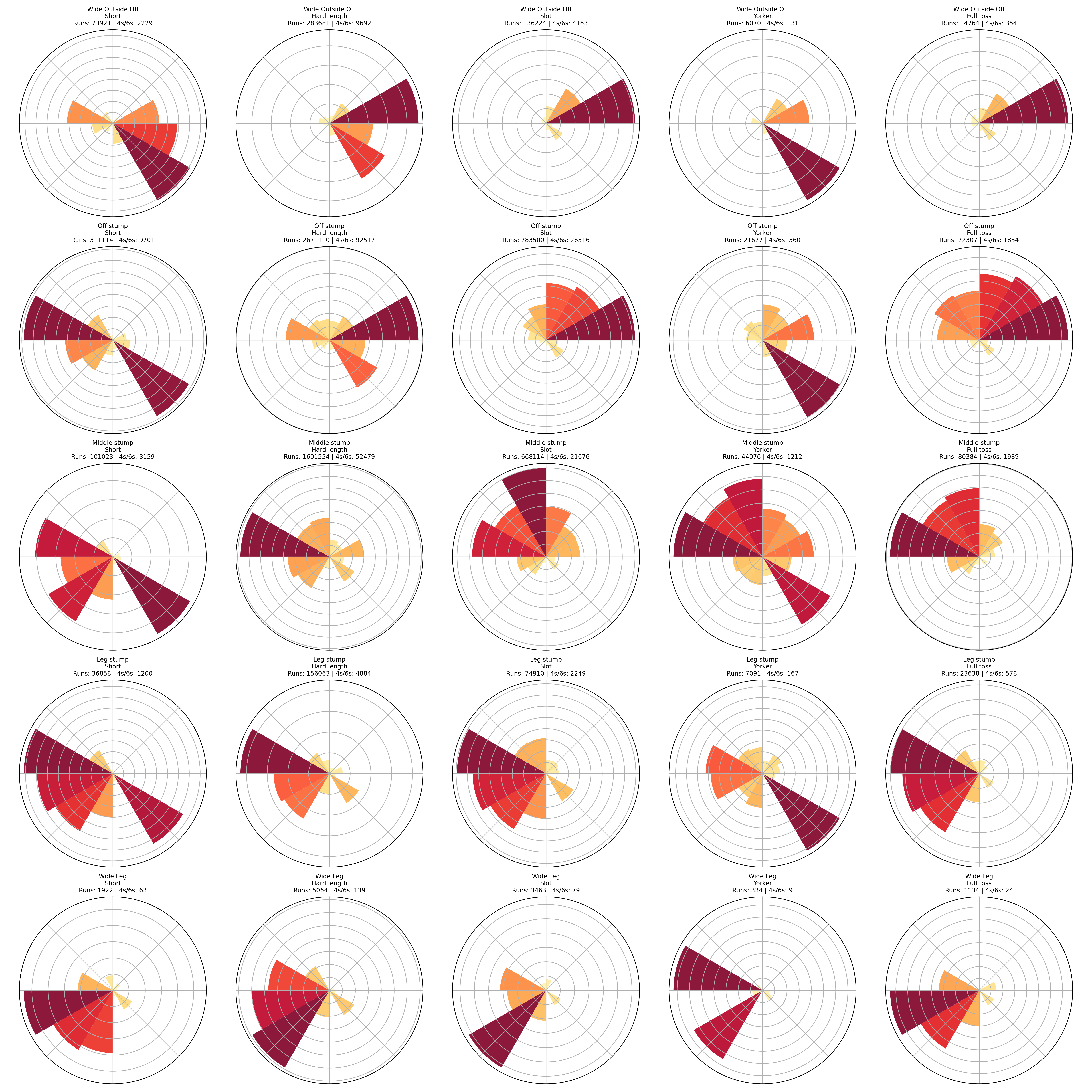
3. The Data Backbone: Discretizing the Wagon Wheel

Before the evolutionary process (the GA) can optimize a field, it needs a "Map" of historical tendencies. Raw coordinates (`wagonX`, `wagonY`) are noisy. To solve this, the engine performs a granular breakdown, binning every shot into specific Line & Length Clusters.

We transform the raw Cartesian data into a Polar Probability Density function. For every combination of Line (e.g., Wide Outside Off) and Length (e.g., Short), we compute the `wagonZone` distribution.

Interactive: Tactical Pitch Map

Select a zone on the pitch to simulate delivery physics.

Popping Crease

Short

Good

Full

Yorker

Full Toss

Select a zone...

0° = Bowler (Top)

Scoring Density Key

High (75%+)

Medium (50%)

Active (30%)

Low (10%)

4. The Genetic Algorithm: Evolving the Field

Field placement is a discrete optimization problem with complex constraints (e.g., Max 5 on Leg Side). Gradient-based methods fail here because "moving" a fielder from Ring 2 to Ring 5 is a non-linear jump, not a smooth gradient.

I implemented a custom Genetic Algorithm that treats the entire field setting as a single Chromosome composed of integer pairs representing [Ring, Sector] for each fielder.

S15

S04

S32

...

S12

Fig 2. Visual representation of the field chromosome. Fielder 1 is at Ring 2, Sector 15.

Accelerating Convergence: Heuristic Seeding

Standard Genetic Algorithms start with random noise. To speed up the solution finding, we employ Meta-Heuristic Initialization. We inject the top historical clusters (derived from the KDE) directly into the initial population ($Pop_{gen0}$). This gives the AI a "head start," allowing it to spend its computational resources refining the exact angles rather than searching the entire ground blindly.

5. The Fitness Function & Powerplay Logic

The fitness function drives the evolution. It is a maximization problem where we reward Wicket Probability ($xW$) and heavily penalize Expected Runs ($xR$).

J(\theta) = (xW_{sim} \times 8000) - (xR_{net}^3 \times 1000) - P_{total}

Baseline Delta Calculation

Before optimization begins, we compute two theoretical states: $xR_{open}$ (No fielders) and $xR_{covered}$ (Perfect coverage). The algorithm works to minimize the delta between the actual field's performance and the theoretical perfect cover.

Constraint Enforcement (The Repair Function)

The math includes strict penalty terms for cricket laws. For example, the Powerplay Penalty ($P_{pp}$) ensures strict adherence to fielding circles:

P_{pp} = \lambda \times \max(0, N_{outside} - N_{allowed})

Where $N_{allowed}$ changes dynamically based on the match phase (2 in PP1, 4 in PP2, 5 in Death). This ensures that any solution violating field restrictions is immediately discarded by the evolutionary process.

Case Study: The 'Perfect' Death Field

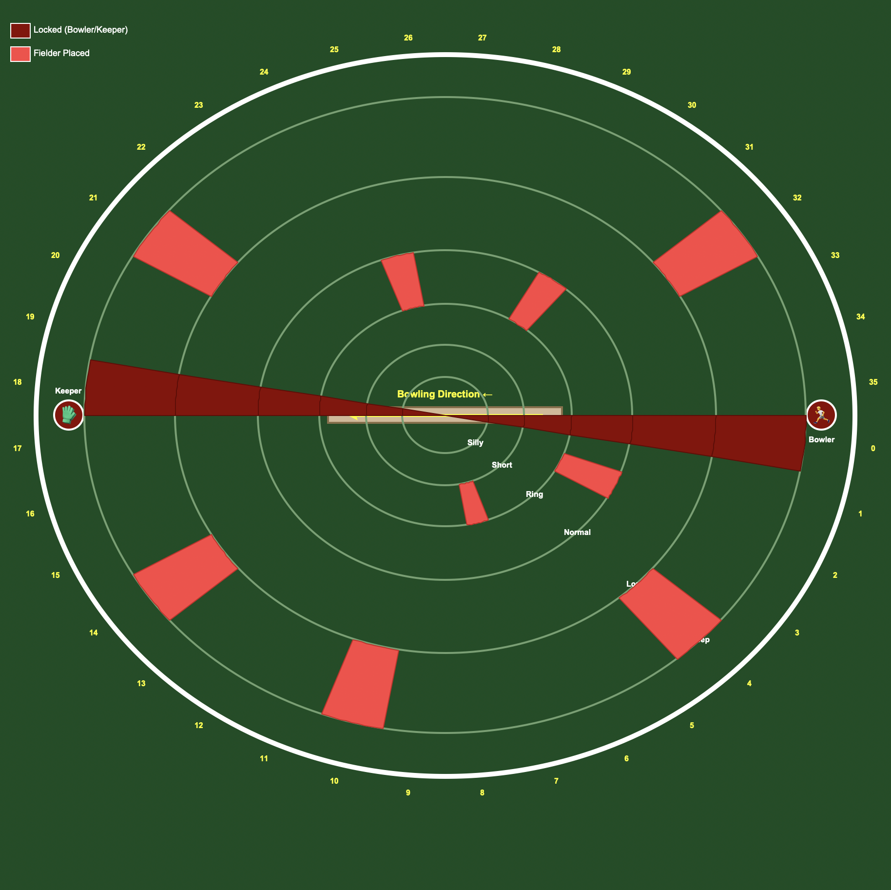
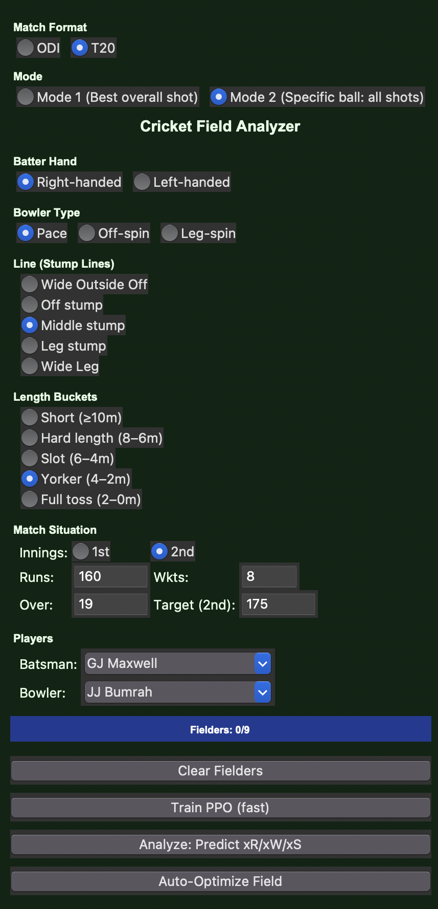
To demonstrate the engine's capability in high-pressure scenarios, we simulated a specific T20 "Death Over" situation. The scenario: 15 runs required off 6 balls. Glenn Maxwell on strike against Jasprit Bumrah. The selected delivery is a Middle-Stump Yorker.

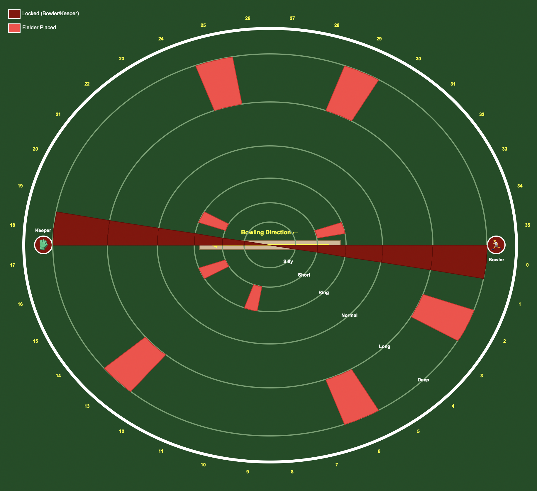
Input Configuration — Fig 3a. The Scenario: 19th Over, Chasing 175.

Optimized Field — Fig 3b. The Output: The "Yorker Trap".

The field that my model suggested (Fig 3b) is a textbook example of modern T20 defensive tactics. Here is why this specific configuration is highly effective:

1. The "V" Lockdown: The engine correctly identified that the most probable "safe" shot against a perfect yorker is the straight drive. It placed fielders deep at both Long-On and Long-Off, creating a double-layered wall down the ground.
2. The Leg-Side Trap: Recognizing Maxwell's aggressive tendency to heave across the line, the simulation maintained Deep Mid-Wicket and Deep Square Leg. It balanced the physics of the yorker (hard to hit) with the psychology of the batter (desperate to score), creating a catching zone for the mistimed slog.
3. The "Missing" Third Man: The AI made a bold tactical choice by removing the deep boundary rider at Third Man. It calculated that the "Reverse Scoop" against a 145kmph Bumrah yorker carried such a high Wicket Probability ($xW > 0.6$) that it wasn't worth wasting a fielder there. Instead, it brought a fielder inside the ring (Short Third Man) to stop the single/edge, prioritizing wicket-taking over boundary prevention.

Validation: The Death Over Stress Test

The raw output below confirms the efficacy of the field shown in Fig 3b. By forcing the Expected Value (EV) of the best possible shot (Straight Drive) down to a measly 0.43, the AI has mathematically tilted the game in the bowler's favor.

Crucially, the xW of 19.6% and the xR of 2.00 runs on the safest shot in the death over implies a dual victory: restricting the batsman to a mere 2 runs is effectively a match-winning outcome on its own, especially when 15 runs are required off 6 balls the pressure created on the batter will be immense, yet the accompanying high dismissal chance suggests the field is not just saving runs, but actively hunting for the wicket. This positive feedback loop between field placement and delivery execution illustrates the power of the Hybrid xR engine in high-stress environments.

user@hybrid-xr-engine ~ % python analyze_maxwell.py

====================================================== 🏏 SHOT PREDICTION ANALYSIS ====================================================== Format: T20 | Phase: DEATH | Over: 19.0 Score: 160/8 Chase: Need 15 off 6 | RRR 15.00 Field Restriction: ≤ 5 outside circle Batsman: GJ Maxwell (RH) | Avg=24.3, SR=148.9 Bowler : JJ Bumrah (pace) | Econ=6.08 Aggression: 100% | Pressure: 90% straight_drive ✓ sec=35 ring=4 COVERED xR=2.00 xW=19.6% EV=0.43 Runs: 0→13% 1→24% 2→41% 3→2% 4→17% 6→4% flick ✓ sec=29 ring=3 open xR=2.12 xW=27.1% EV=-0.05 Runs: 0→16% 1→28% 2→22% 3→4% 4→26% 6→4% on_drive ✓ sec=35 ring=3 COVERED xR=1.86 xW=24.3% EV=-0.09 Runs: 0→19% 1→23% 2→38% 3→2% 4→16% 6→3% cover_drive ✓ sec=06 ring=5 COVERED xR=0.67 xW=41.2% EV=-2.62 Runs: 0→69% 1→15% 2→6% 3→1% 4→8% cut ❌ NOT RECOMMENDED xR=0.42 xW=36.5% EV=-2.50 Runs: 0→82% 1→7% 2→4% 3→1% 4→5% late_cut ❌ NOT RECOMMENDED xR=0.42 xW=36.5% EV=-2.50 Runs: 0→82% 1→7% 2→4% 3→1% 4→5% sweep ❌ ILLEGAL xR=0.18 xW=46.1% EV=-3.51 Runs: 0→91% 1→3% 2→4% defend ❌ ILLEGAL xR=0.06 xW=50.7% EV=-3.99 Runs: 0→95% 1→4% leave ❌ ILLEGAL xR=0.04 xW=99.0% EV=-6.28 Runs: 0→100% 1→0% 🏆 BEST LEGAL SHOT: STRAIGHT_DRIVE xR=2.00 xW=19.6% EV=0.43

Match Analysis & Case Studies

Putting the Engine to the Test

Theoretical physics and AI optimization are only as good as their real-world application. In this section, we unleash the Hybrid xR engine on some of the most iconic players and high-pressure situations in cricket history to see if the math validates the magic.

Hybrid xR has multiple applications ranging from a analysis model to a standalone performance metric. Let's explore them in action.

Case Study 1: The First-Over Massacre (Abhishek Sharma vs Jacob Duffy)

Today’s T20 game (January 31st, 2026), India vs New Zealand, was completely dominated by India. After 20 overs, India set a massive 272-run target for New Zealand.

There was one player who absolutely dismantled New Zealand’s prime bowler, Jacob Duffy, in the very first over itself. Known for hitting sixes and boundaries from the start, he doesn’t believe in wasting time. Any guesses who? You guessed it right: Abhishek Sharma.

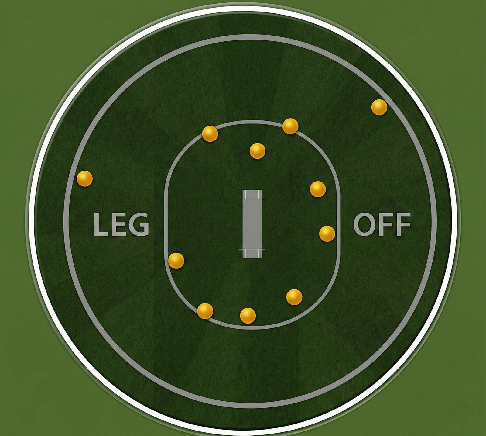
One such first-over massacre was observed today. Let's look at the field set for him, and two specific instances that occurred in that very first over.

Before proceeding, one caveat: My model doesn’t handle sixes perfectly yet. Because it’s not a full 3D model, it doesn’t fully calculate the z-axis (elevation). Let's see how it performed regardless.

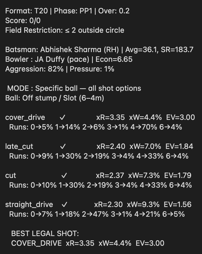
Actual Field Set for Abhishek Sharma — Fig 4a. The actual field set by New Zealand against Abhishek Sharma in the first over.

Instance 1: 0.2 Overs (Score: 0/0)

On the 3rd ball of the match, Duffy bowls an off-stump slot ball (6-4m). Abhishek isn’t one to miss out on these it goes for a six.

So, what does the model have to say? My model correctly identified that the cover_drive is the most valuable shot in that exact setting. Credit to Abhishek for executing it perfectly. In the output below, the 4-hitting probability for this shot is a massive 70%, which strongly suggests the model is thinking in the right direction.

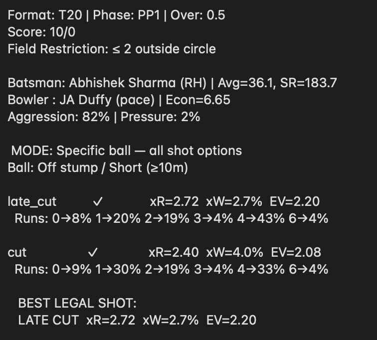
Hybrid xR Terminal Output for 0.2 Overs — Fig 4b. Terminal analysis for the 0.2 off-stump slot delivery.

Instance 2: 0.5 Overs (Score: 10/0)

He wasn’t content with the 10 runs already on the board. On the last ball of the over, Duffy bowls a short ball on off-stump (≥10m). Abhishek isn’t shy to late-cut that ball, picking up a four through the third-man region.

What does the model say? The model correctly flagged late_cut as the most valuable shot. The probability of hitting a 4 is 43%. This reduced probability makes sense because there’s a deep third man in place, but at that pace, the fielder can only watch the ball run to the boundary.

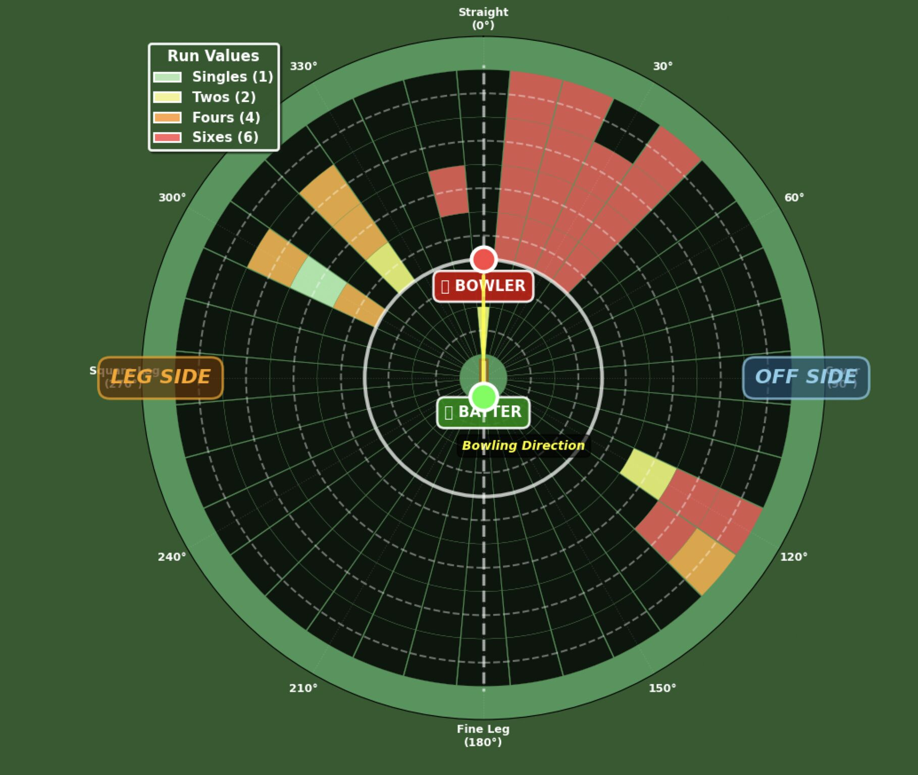
Hybrid xR Terminal Output for 0.5 Overs — Fig 4c. Terminal analysis for the 0.5 off-stump short delivery.

Visualizing Intent: The Scoring Heatmap

To understand why the engine prioritizes shots like the cover drive and late cut, we can look at its directional intent essentially, a visualization of how the model "thinks."

The heatmap below reflects the specific areas of the field the model is actively exploring to identify key scoring regions for Abhishek Sharma. By mapping out projected run values across the field, it perfectly illustrates the intersection of his aggressive hitting profile and the spatial gaps available to him.

Abhishek Sharma Scoring Heatmap — Fig 4d. Radial heatmap showing the model's projected scoring zones and directional intent for Abhishek Sharma.

The Counter-Attack: Running the Bowler's Engine

While running the bowler’s engine to minimize runs and suggest a defensive field for that 0.5 delivery, the model made two distinct adjustments to the original field:

It pulled Third Man slightly finer.
For some reason, it moved Square Leg a bit squarer.

This algorithmic adjustment reduced the 4-hitting probability down to 29%, showing that even subtle field changes can meaningfully impact outcomes and choke the Expected Runs (xR).

Case Study 2: The Perfect Trap (Josh Inglis vs Zimbabwe's Masterclass)

Yesterday (February 13th, 2026), the cricketing world witnessed a massive upset as Zimbabwe defeated Australia by 23 runs. Honestly, looking at the tactical setups, I knew it would be a tough matchup.

In T20 cricket, setting a solid foundation is all about the opening partnership. Having that broken in the very first over creates massive pressure on the middle order and that is exactly what happened here.

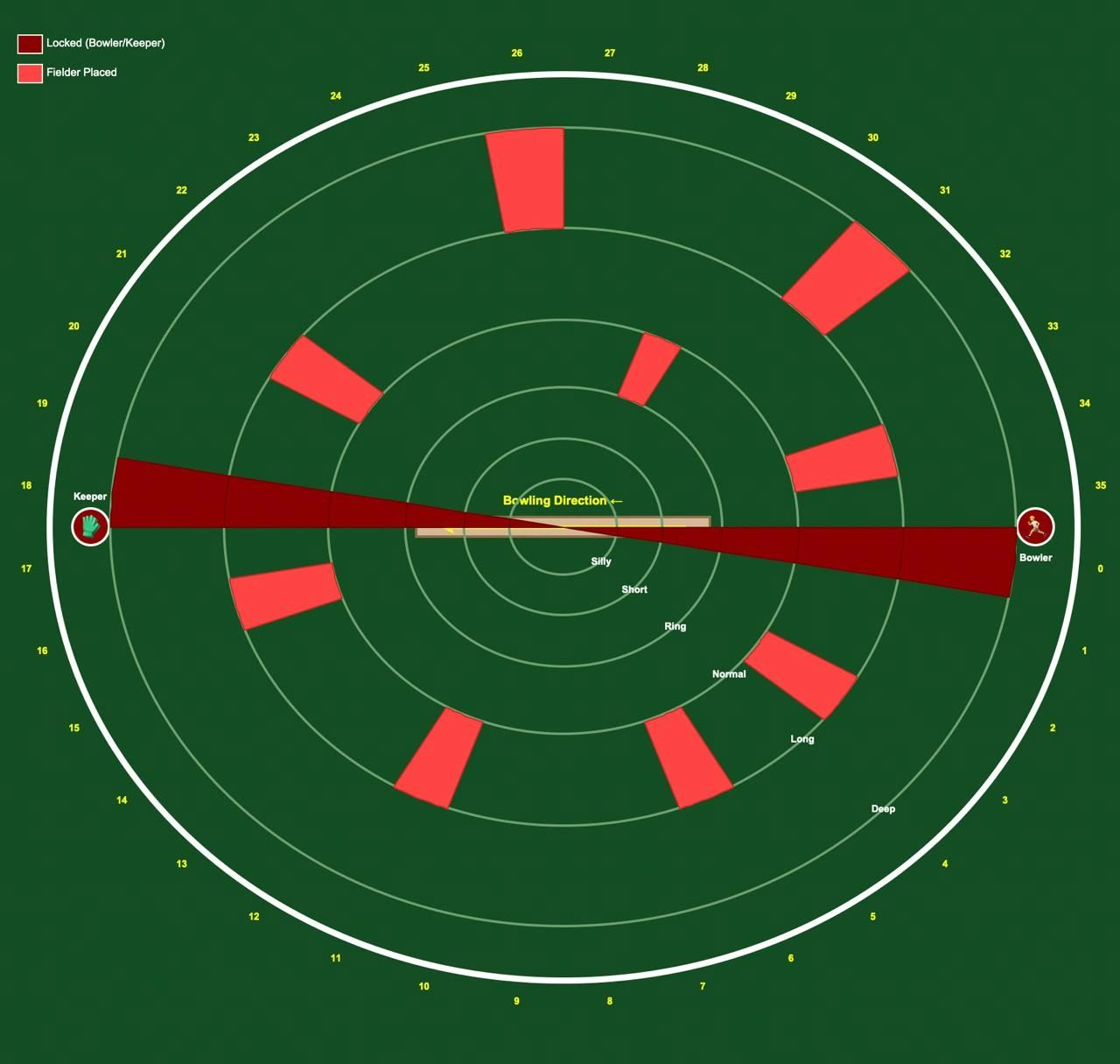
The Setup: Cramping the Batter

Let’s analyze Josh Inglis’s shot with respect to the field set and the specific delivery. Blessing Muzarabani bowls a middle-leg short ball (≥10m). As we can see in the match snapshot below, Inglis’s trigger movement is practically non-existent. He remains stationed on the leg stump, which ends up completely cramping him for space.

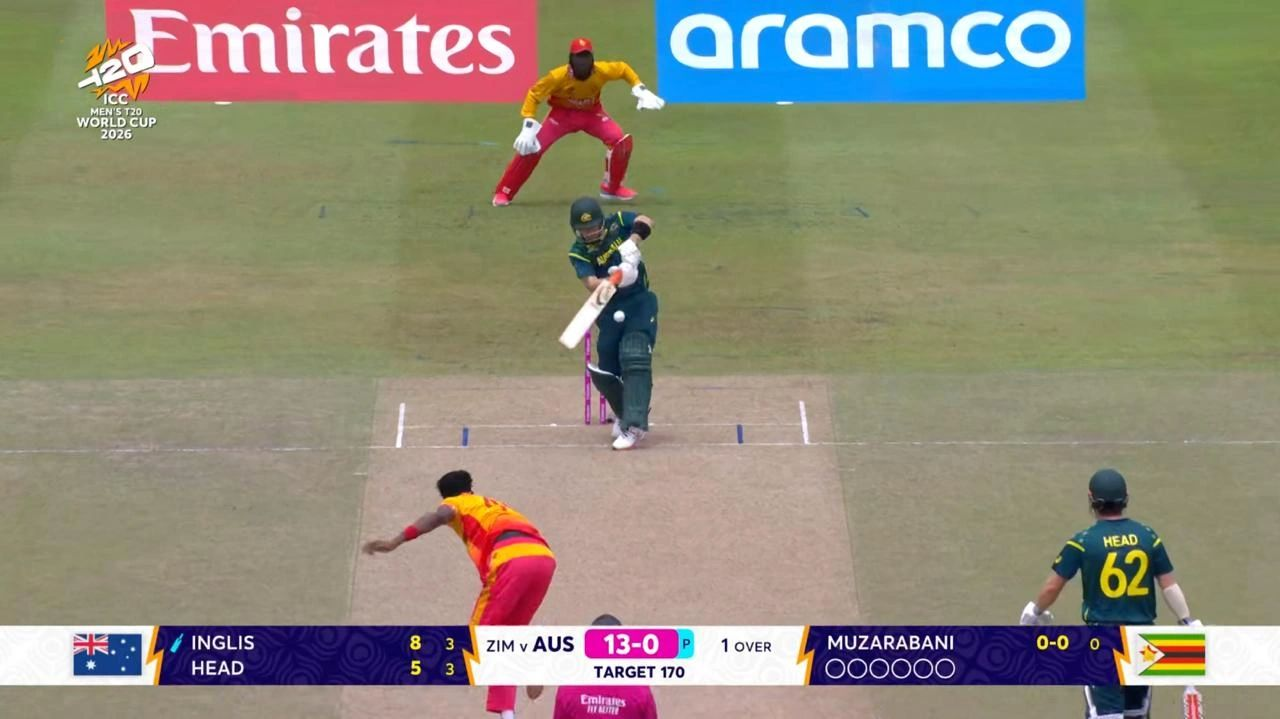
Josh Inglis cramped for room — Fig 5a. Inglis cramped on the leg stump against Muzarabani's short delivery.

Because he is cramped, he is physically forced to play the shot squarer directly into the hands of the fielder specifically placed there. I’d call it the "perfect trap."

Zimbabwe Field Setup for Inglis — Fig 5b. Zimbabwe's field map showing the square leg trap.

The Hybrid xR Verdict

Let’s see what the model had to say about this specific delivery and field configuration.

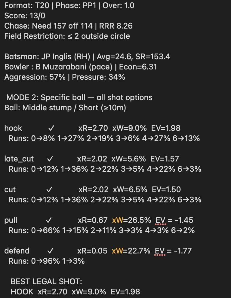
Hybrid xR Terminal Output for Inglis — Fig 5c. Terminal analysis showing the extreme risk of the pull shot.

The engine correctly identified that playing the pull shot here is incredibly dangerous. The Wicket Probability (xW) spikes to a massive 26.5%, and the Expected Value (EV) plummets to -1.45. In a real-match scenario, that mathematically translates to a highly likely dismissal.

Conversely, the model analyzed that the hook would be the best possible shot (xR=2.70, xW=9.0%). From a biomechanical perspective, this makes perfect sense. If Inglis had incorporated a pre-delivery trigger movement bringing his back foot toward the middle-off region before making contact, the area behind square leg would have opened up, allowing for a high-EV hook shot.

🔥 Tactical Brilliance

In other words, Zimbabwe showed their absolute class by analyzing the shortcomings of Inglis’s static stance and essentially cramping him out of his safe scoring angles. A true tactical masterclass by Zim.

Case Study 3: The Player Persona (Ranking and Classifying players in the Super 8 Match: India Vs West Indies)

This is one of the most powerful applications of Hybrid xR. Built on top of the Hybrid xR engine is a framework called “Player Persona”, designed to evaluate player performance for both batsmen and bowlers. It judges players not just on static scorecards, but on the process behind the outcome factoring in shot quality and biomechanical feasibility relative to the field set.

This now means, a player getting lucky boundaries, may not be rewarded as well, compared to someone who scores with pin point precision and control.

The Test Case: Super 8 (IND vs WI)

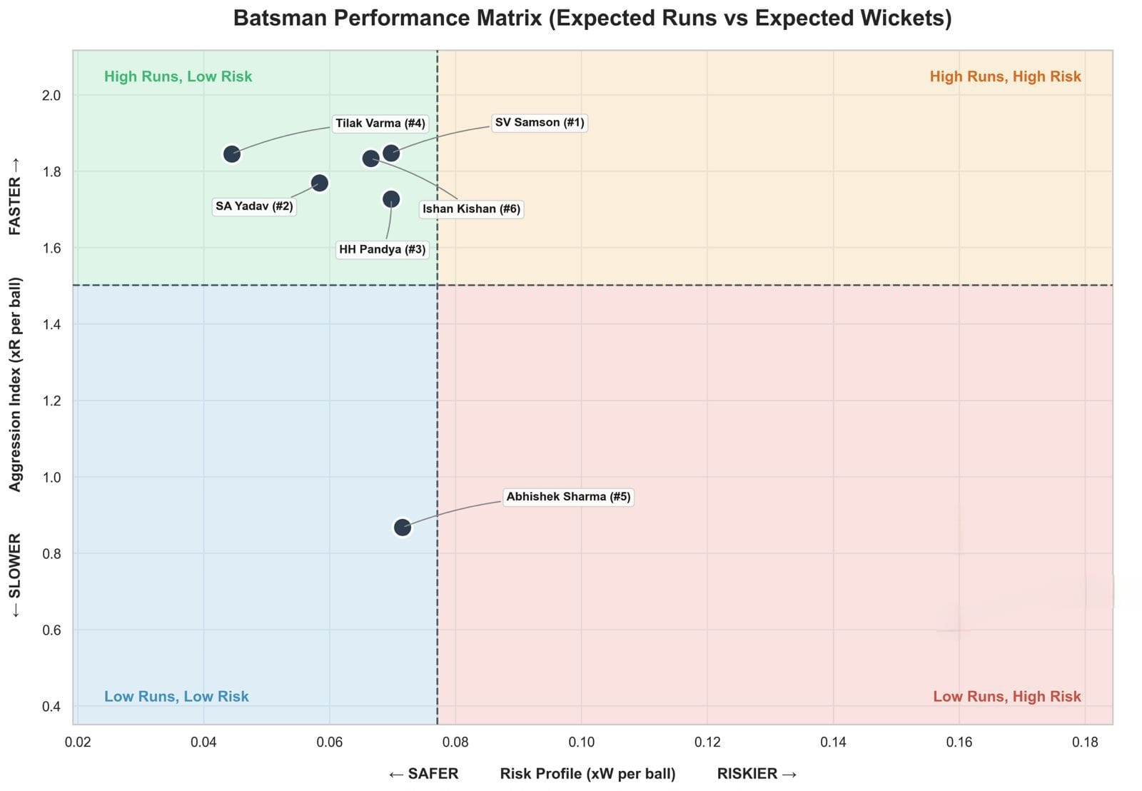
Looking at the data, the framework clearly separates the elite performers from the rest based on underlying metrics rather than just surface-level stats.

For instance, in the Batsman Matrix, Sanju Samson and Suryakumar Yadav sit firmly in the elite "High Runs, Low Risk" quadrant, proving they generated a massive True Strike Rate (xR per ball) while keeping their wicket probability mathematically controlled. On the flip side, the model accurately captures batting struggles, cleanly mapping Abhishek Sharma into the "Low Runs" territory, highlighting an inability to generate high expected value per ball on that specific day.

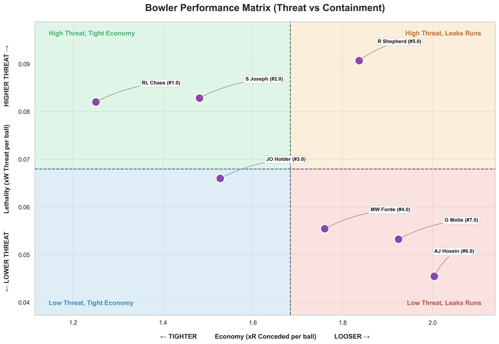
On the bowling side, Roston Chase and Alzarri Joseph emerge as the ultimate weapons in the "High Threat, Tight Economy" zone, maximizing their lethality while effectively choking the batters' expected runs. Conversely, the model exposes bowlers like Romario Shepherd, who despite being a high threat, leaked runs at a high expected rate, placing him in the high-risk quadrant

The attached images show the Player Persona analysis of the Super 8, do-or-die match, India vs West Indies.

Fig 6a. Batsman Performance Matrix mapping Aggression Index vs Risk Profile.

Fig 6b. Bowler Performance Matrix mapping Lethality vs Economy.

Some rankings might feel off at first glance. And that’s the point.

Because while runs and outcomes matter, how those runs come matters even more. Cricket isn’t just about how many runs you score. It’s about how you score them.

Intelligent Batsman and Bowler Persona

Beyond the Scorecard: Separating Process from Result

Traditional cricket statistics suffer from Result Bias. If a batsman hits a reckless heave for six, the scorecard calls it a success. If they play a perfect cover drive that finds a diving fielder, it's an inferior shot.

The Persona model: It's an application of the Hybrid xR engine, which create metrics that capture intent and accuracy of a player, instead of the absolute result. It is designed to strip away luck and reveal the "True Skill" of a player. It does this through a three-layer intelligence stack.

1. The Dynamic Wicket Engine (Marginal Markov Cost)

In T20 cricket, wickets are a currency. Our model leverages an Absorbing Markov Chain to calculate the exact Expected Runs Remaining ($ERR$) from any state.

Defining the 3D State: In this framework, the State Space ($S_i$) of the innings is a three-dimensional matrix defined by: $S_i = (b, w, r)$, where $b$ is balls remaining, $w$ is wickets in hand, and $r$ is current runs scored.

This expectation is driven not just by the Opportunity Cost of these remaining deliveries, but crucially by the Current Run Rate (CRR), ensuring the transition matrix adapts to real-time match momentum:

E[S_{b,w,r}] = \sum_{x \in \{0..6\}} P_t(x) \cdot E[S_{b-1, w, r+x}] + P_t(W) \cdot E[S_{b-1, w-1, r}]

Using this dynamic state matrix, we can calculate the exact Marginal Cost of a dismissal at any given second, split logically between setting a target and chasing one.

1st Innings: The True Opportunity Cost

When setting a total, the penalty for getting out is simply the absolute drop in the team's Expected Final Score. Because current runs ($r$) remain static when a wicket falls, the penalty is precisely the difference between the two 3D Markov states.

Penalty_{1st} = E[S_{b,\ w,\ r}] - E[S_{b,\ w-1,\ r}]

2nd Innings: The Contextual Forgiveness

In a chase, the target dictates the required risk. We apply a Markov Forgiveness Factor. If the math states the team is heavily projected to lose (where Expected Runs Remaining, $E[S_{b, w, r}] - r$, is much lower than Runs Needed), the batsman is not heavily penalized for getting caught while attempting a necessary, high-risk shot to bridge the gap.

Penalty_{2nd} = Penalty_{1st} \times \left( \frac{E[S_{b,\ w,\ r}] - r}{\text{Runs Needed}} \right)

This dynamic marginal cost ensures that the penalty remains high during the Powerplay (when resource preservation is vital) and collapses rapidly during the Death Overs. This "Strategic Intelligence" is what allows the engine to correctly rank a high-risk finisher above a low-risk anchor in an impossible chase.

2. The 360-Degree Leaderboard

To provide a full tactical profile, we evaluate every player across five distinct dimensions. This allows a coach to pick the right "tool" for the specific match situation:

True Strike Rate (xR/ball)

Expected scoring speed based purely on delivery physics and intent, removing the noise of lucky boundaries.

Cricketing Brain (% Smart Shots)

Measures decision-making by checking if the shot played was biomechanically optimal for that specific line and length.

Scoring Efficiency (Execution)

The delta between Actual Runs and Expected Runs. This highlights players who are physically beating the math.

Boundary Threat

The mathematical probability of finding the rope on any given ball based on field gaps and power profile.

Master Metric: Risk-Adjusted Impact

The ultimate scouting value. It balances aggressive intent against the Dynamic Wicket Penalty. This is how we identify players who score fast when it matters, without throwing their wicket away recklessly.

3. Batsman Persona: The Runs-vs-Wicket Matrix

Raw data tells you how many runs a player might score. Persona tells you how good or bad a batter was spanning over his entire innings. We use K-Means clustering to analyze the spatial relationship between Aggression (xR) and Risk (xW), segmenting the field into four tactical archetypes:

HRLW: High Runs, Low Wickets

High Reward, Low Wicket. These are your match-winners. They maximize scoring while maintaining mathematical safety.

HRHW: High Runs, High Wickets

High Reward, High Wicket. High-variance players used to break a game open. They score fast but are mathematically likely to get out.

LRLW: Low Runs, Low Wickets

Low Reward, Low Wicket. Defensive specialists. They don't score fast, but they are vital for stabilizing an innings after a collapse.

LRHW: Low Runs, High Wickets

Low Reward, High Wicket. Players struggling with form or shot selection. Mathematically, they are a drain on the team's resources.

4. Bowler Persona: The Threat-vs-Containment Matrix

We apply the same logic to bowlers, mapping Lethality (xW) against Economy (xR Conceded). This allows us to move beyond basic economy rates and identify four distinct bowling archetypes:

HTLR: High Threat, Low Runs

High Threat, Low Runs. High wicket probability paired with extreme run containment. The gold standard of bowling.

HTHR: High Threat, High Runs

High Threat, High Runs. Bowlers who hunt wickets aggressively but are prone to leaking boundaries.

LTLR: Low Threat, Low Runs

Low Threat, Low Runs. Pressure specialists. They dry up runs to force mistakes at the other end.

LTHR: Low Threat, High Runs

Low Threat, High Runs. Bowlers struggling for both rhythm and penetration. In our model, they represent the highest run-leak risk.

Real-World Applications

How could this framework be utilized at the highest levels of the sport?

Optimized Squad Selection: With sufficient ball-by-ball player data, teams and franchises can use these matrices to build perfectly balanced lineups. It shifts the focus from simply picking players with high averages to selecting the exact tactical archetypes required to maximize overall team performance.
Context-Aware Player Rankings: Current official player rankings (like the ICC rankings) rely heavily on static scorecards, judging players primarily by absolute runs, strike rates, and raw opposition strength. The Player Persona framework offers a much fairer, context-aware method to evaluate a player's true skill and impact, completely removing the element of "scorecard luck."

Intelligence in Action

"Theory is the foundation, but execution is the prize. To see how these 360° metrics decode the real world matchups..."

Conclusion

This model moves cricket analytics from "What happened?" to "What will happen?". By mathematically formalizing the concepts of Intent, Pressure, and Physics, we can assign a definitive value to every decision on the field, separating the process from the outcome.